Entrance I: group analysis(consistent with the original version)
Quick introduction to analysis procedure
The following table summarizes all of the species groups gathered by agriGO v2.0 at present:
| Category | Classification | Counts |
| Plant | ||
| Brassicaceae | 12 | |
| Poaceae | 29 | |
| Malvaceae | 6 | |
| Fabaceae | 16 | |
| Solanaceae | 12 | |
| Rosaceae | 5 | |
| Medicinal plant | 12 | |
| Tree | 29 | |
| Algae | 18 | |
| Animal | ||
| Fish | 20 | |
| Aves | 11 | |
| Amphibia | 3 | |
| Insecta | 56 | |
| Mammalia | 58 | |
| Fungi | Sordariomycetes | 5 |
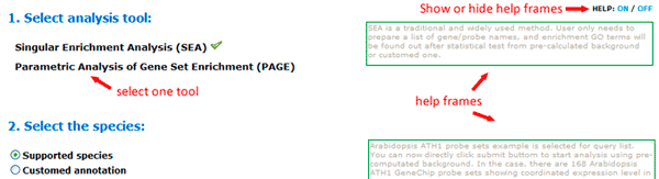
You should choose one tool to go forward. At the right side, several frames containing annotation text are interactive. The content will change depending on exact parameters you chose. You can make the help frames show or hidden by using HELP buttons at top-right of the page.
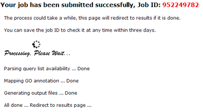
After submitting your job, the agriGO will pre-check the validity of your upload data. If your job is submitted successfully, a job ID will be given. Since the analysis process could take a while, you may close the waiting page and use the job ID to check the work later. Please note that results of your jobs will be stored on our server for THREE DAYS. After 7 days all information of the job will be deleted. If you want elongation contact me.
The agriGO provides different ways to browse results of different tools. Some of them are flexible but you may need some specific setting to make them to castor to your own demands. And detailed introduction to these tools in the manual in the following will help you to achieve it.
How to use Singular Enrichment Analysis (SEA) analysis?
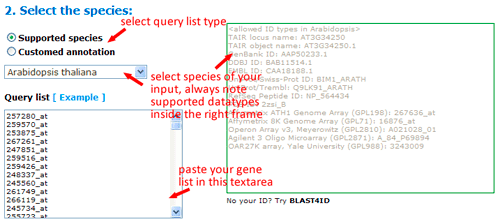
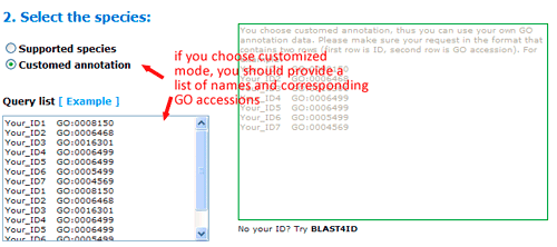
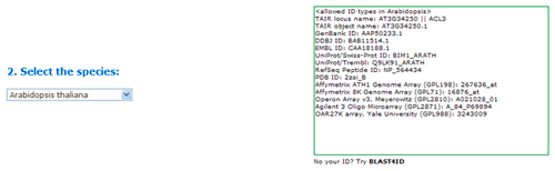
To use SEA analysis, you should firstly select the type of your query list, either single names or names with GO accession. If you choose using supported species in agriGO, you only need to provide a list of sequence identifiers. It should be noted that you would better select species and check all allowed ID types of corresponding species, then submit your IDs. Only allowed IDs are suitable to be analysis in this type mode. And you can mix your IDs from different types. Just ensure they are allowed IDs.
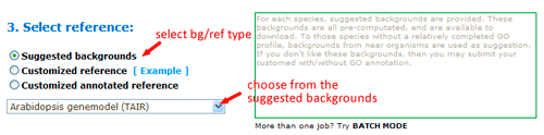
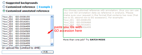
Now you can set the background or reference. There three types: suggested backgrounds, customized reference and customized annotated reference. The default parameter is using suggested backgrounds. For each species, agriGO will give all possible the background types. To those species without a relatively completed profile, backgrounds from neighbored organisms are suggested. Users can select based on their practical need, otherwise use customized reference.

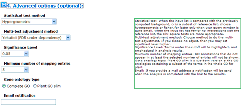
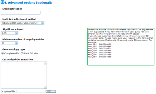
The advanced options are optional but quite important. These options are default hidden, and need to one click to make them visible. In SEA analysis, there are three statistical test methods: hypergeometric, chi-square and fisher test.
When the input/query list is compared with the previously computed background, or is a subset of reference list, choose hypergeometric or fisher. When both of your query list number and reference list number are quite small, you may better choose fisher test. When the input/query list has few or no intersections with the reference list, the Chi-square tests are more appropriate. Next you can choose method to do the multi-test adjustment. Seven adjustment methods are available here, including: Yekutieli (FDR under dependency), Bonferroni, Hochberg, Hochberg (FDR), Hommel, Holm, False Discovery Rate. Though I would suggest perform adjustment test, you truly can turn off it and use no adjust. While you choose no adjust, then you may set significant level below higher. Terms under the cutoff of the significant level will be highlighted, and emphasized in analysis results, and it will affect your test output.
Minimum number of mapping entries means that GO annotations that do not appear in at least the selected number of entries will not be shown. In other word, higher you set the number, more entries needed to make one GO term appear in the analysis result.
Gene ontology type: Plant GO slim is a cut-down version of the GO ontologies containing a subset of the terms in the whole GO for plant.
Last, if you provide a mail address, a notification will be send when the analysis is completed with the link to the results. Providing a email address is optional to SEA analysis, because it is very fast.
Singular Enrichment Analysis (SEA) Results
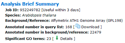
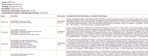
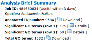
A brief summary of your job will be given. The job ID is useful within 7 days. A file containing all entities in the query list that can be annotated by GO associated with descriptions is able to download.
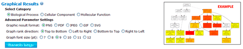
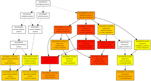
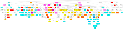
In this part, you can browse the hieratical graph result. Note that the graphical result was generated as separate graphs for each of the three GO categories, namely biological process, molecular function and cellular component. After select the category, uses can specified their favorite output format, graph rank direction and font size. The result format means which output format you preferred. The rank direction is used to define the direction in your output, for instance the direction in the example image is 'top to bottom' And the font size is self-evident that user can set smaller size if there are many nodes in their result.
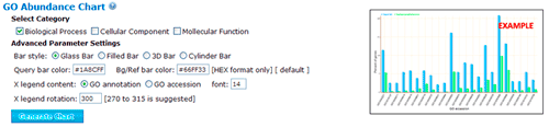
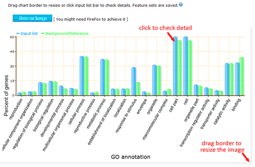
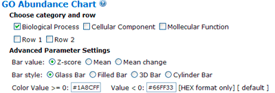
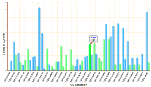
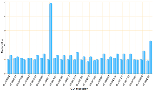
The terms selected here are children terms of root one (or called secondary level terms) or significant terms of secondary level terms. Thus, the bar chart gives user a brief portray since the GO terms are relatively general description. Similar to the procedure of graphical result, user should specified their parameters before create the GO abundance chart. User can try these setting to obtain favorite view of the chart bar. Note the setting you used will be recorded in your cookie and these settings will be default ones in your future jobs. In other word, you may try several times and make your last attempt as your own features.
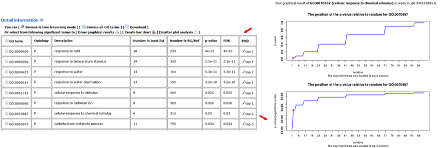
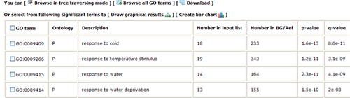
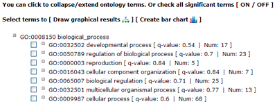
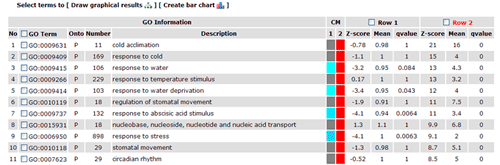
In this part, detailed information is given. All GO significant terms will presented in the following table. And you can browse the GO terms using tree traversing mode (we will discussed it later), or can browse all GO terms in the similar type table, or just the data. User can select terms to draw graphical result or create bar chart. Please note that the parameters used in graph or chart generating is fetched from your cookie, and your cookie will be set or changed when you generate graphical results or GO abundant chart which has been mentioned in part 2 and 3. While it will make you a bit trouble if you would like adjust the images created here to redo the part 2 or 3 work once more to change the settings. Click the checkbox left to 'GO term' can select all GO terms at one time.
How to use Parametric Analysis of Gene Set Enrichment (PAGE)
Firstly, you should choose the species for your query data. Please make sure that identifiers in your input should be one of datatypes inside the right information table. If your identifiers are not stored in agriGO, there is another two ways: one is provided your own GO annotation file, the other is to use our BLAST4ID service.
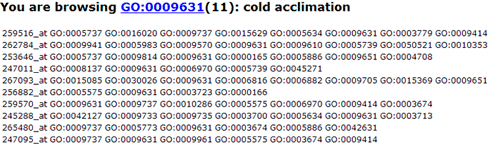
In PAGE analysis, user should pay more attention to input data. As presented in the following image, as least two rows must be provided. The first row is sequence identifiers, and followings are numerical value. The numerical value is fold change (FC) or log2-transformed FC value (latter preferred) of the identifiers' expression under different condition. If you do not have expression data, then SEA may be the alternative choice. In agriGO example, there are 3 rows in this example. First row is ATH1 probeset name, the second row is expression fold change (FC) value of cold treatment to CK(cold/CK) after half hour. Third row is expression FC of cold/CK after 24 hour cold treatment. Only 600 probesets are in the quick example for the fast load of the HTML page. To obtain a full view of PAGE method, you can download the full example file and explore the following analysis procedure.

Next you can choose method to do the multi-test adjustment. Seven adjustment methods are available here, including: Yekutieli (FDR under dependency), Bonferroni, Hochberg, Hochberg (FDR), Hommel, Holm, False Discovery Rate. Though I would suggest perform adjustment test, you truly can turn off it and use no adjust. While you choose no adjust, then you may set significant level below higher. Terms under the cutoff of the significant level will be highlighted, and emphasized in analysis results, and it will affect your test output. Minimum number of mapping entries means that GO annotations that do not appear in at least the selected number of entries will not be shown. In other word, higher you set the number, more entries needed to make one GO term appear in the analysis result.
Gene ontology type: Plant GO slim is a cut-down version of the GO ontologies containing a subset of the terms in the whole GO for plant. If you can also upload your own customized GO annotation file once your identifiers are not accepted directly by agriGO. The file's size is limited to 4MB.
Parametric Analysis of Gene Set Enrichment (PAGE) Result

Entrance II: single species analysis
How to perform a Batch Singular Enrichment Analysis (SEA)
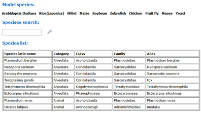
You can select one of your species of interest or model species from the table for the first time to use agriGO v2.0. We have provided 10 kinds of model species related to the new classification system across different categories. The model plant Arabidopsis thaliana has been used as an example to illustrate the process.
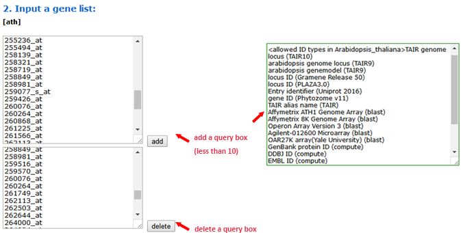
To use the SEA tool, you should first select the type of query list. You can input multiple query lists at a time by adding gene list boxes.
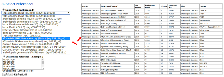
Now, you can set the background or reference. Suggested backgrounds and customized references are provided. The default parameter uses the suggested background. For each species, agriGO v2.0 will provide all of the possible background types.
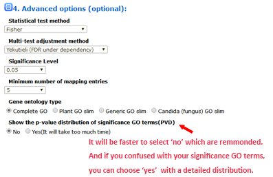
The advanced options are optional but important. These options are hidden by default, and need to be clicked to make them visible. In the SEA analysis, the new option PVD (p-value distribution) was added. We used PVD to display the distribution of p-values of significant GO terms from query and random datasets. The line chart can illustrate the location and the percentage among the 99 random results. It is not calculated by default nor recommended for the first analysis.
Batch SEA results:
All of the successful job IDs are displayed in the analysis results. You can run a SEACOMPARE by selecting job IDs.
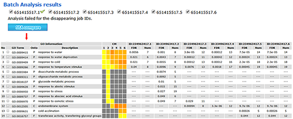
When the PVD option is selected as 'yes', a new column named PVD will appear in the 'Detailed information', in which two distribution line charts with different Y-axes (normal and logarithmic scales) for each significant GO term will be present.